Excel chart overlapping bars
Add a Stacked Bar Chart to your Excel spreadsheet using the Chart menu under the Insert tab. In a certain range.

Tableau Tip Tuesday How To Create Grouped Bar Charts Bar Chart Chart Data Visualization
The chart is constructed by selecting the orange shaded cells Grade Min and Span and inserting a stacked column chart top chart below.
. Data Bars Intro. However you can add data by clicking the Add button above the list of series which includes just the first series. Task description Start date End date Duration.
How to add secondary axis in Excel Column Chart without overlapping bars. To eliminate overlapping. On the far righthand side select the Change Chart Type icon and hover over the Line graph option.
In the screen shot below conditional formatting data bars have been added to a sales. Answer 1 of 3. Change the font color of Spain to red and bold.
Half of the labels are illegible. If I let the. Lets see how to format the charts once inserted.
The next step is to make it look like a proper Gantt chart by formatting it. Check UpDown Bars option. Then click into Chart Design on the menu bar on top of your Excel spreadsheet.
See how to make a histogram chart in Excel by using the Histogram tool of Analysis ToolPak FREQUENCY or COUNTIFS function and a PivotTable. Select the data series to plot on the second axis then click the Chart Layout sub-tab that appears after the chart is selected. Maybe Excel secretly hates you.
Now down to the nitty-gritty. Align the pie chart with the doughnut chart. Add chart title and.
In the Format Axis pane under Axis Options type 1 in the Maximum bound box so that out vertical line extends all the way to the top. Fix up the chart bottom chart below by deleting the legend formatting Min to use no fill and Span to use a light fill color and setting a gap width of 50 or 75. In the Chart Type dropdown menu next to Series Pointer the outer circle choose Pie.
In Excel 2013 click the plus icon beside the chart click on the right-facing arrow beside Axes and check the Secondary Horizontal box. Select any series in the chart and then in the Format Data Series pane under Series Options set the Gap Width to 0. Learn how to create an actual vs budget or target chart in Excel that displays variance on a clustered column or bar chart graph.
You should now see the formatting options on the right of your screen. To create a Gantt chart in Excel that you can use as a template in the future you need to do the following. Select the first line graph option that appears as shown below.
Fill Between Overlapping Regions. We just need to get the data range set up properly for the percentage of completion progress. Why not just call it Make the Bars Wider.
Includes a step-by-step tutorial and free workbook to download. Old versions of Excel had Invert if Negative with a default negative fill color of white. Here you can see all series names Delhi Mumbai Total and Base Line.
The bars in a bar chart will end up overlapping so use another format such as a line graph. How to Add Data Bars. The second chart shows the plotted data for the X axis column B and data for the the two secondary series blank and secondary in columns E F.
But whenever I try to move one series of data on secondary axis. Adjust the size of the chart Height 51 and Width 39. One of the options is to Show the Legend without Overlapping the Chart.
Right Click on the Axis title Then click on Format Axis You will find the Format Axis dialogue box In the Axis position option click on categories in reverse order. Select the inserted chart and then press Ctrl1 a shortcut for formatting the chartThis will provide a sidebar next to the chart with different options to fill the bars will different colors change the background texture etc. In this version of Excel showing data in two different ways is not available but you can add a second axis.
Change chart type of Total and Base Line to line chart. To remove an unwanted legend entry click once on the legend to select it then click again on the legend. Build a line chart.
Thanks for visiting PHD btw the line charts are there just load the template and convert the chart type from bar chart to line chart the colors would adjust automatically they should let me know if this doesnt work. Excel adds a secondary vertical axis along the right edge of the chart. Set up a helper column.
Mac Excel 2011. A vertical line appears in your Excel bar chart and you just need to add a few finishing touches to make it look right. I have now tried to fill the bars below the XY-chart using this post.
Click on the plus sign of upper right corner of graph. Your chart is ready showing both the number of shoes sold and percent according to. Youll see a black Bars connecting Total and Base Line nodes.
Only problem is when I add a new chart for the horizontal bars I use Stacked Area it seems to fill the area within the pointers and not the whole chart. Ive added data labels above the bars with the series names so you can see where the zero-height Blank bars are. Learn how to display the variance between two columns or bars in a clustered chart or graph.
In Excel 2007 you had to apply a gradient fill with an insane gradient setting. Check the Secondary Axis box next to Series Pointer and click OK. The blanks in the first chart align with the bars in the second and vice versa.
Change the Fill color of the bars to light grey and that of Spain to red. How to Create the Progress Doughnut Chart in Excel. Right off the bat create a dummy column called Helper column F and fill the cells in the column with zeros to help you position the timescale at the bottom of the chart plotStep 2.
Your data is now on the stacked bar chart in blue and orange. Now select the Total line. On the blue section of the bar you need to right-clickThen click on Format Data Series.
List your project data into a table with the following columns. First right-click on the newly created outer chart and select Change Series Chart Type. If cells contain numbers you can add conditional formatting data bars to show the differences among the amounts.
In other words a histogram graphically displays the number of elements within the consecutive non-overlapping intervals or bins. You can reverse the order of the stacked bar chart in Excel with the following steps. Excel means the width of the gap between two of those blue bars.
Watch this short video to see how to set up data bars in a cell and the written instructions are below. Select Series Data. Getting the bars wider involves a super geeky technical-sounding Excel move reduce the gap width.
We have different options to change the color and texture of the inserted bars. Free Excel file download. Here is the chart after running the routine without allowing any overlap between labels OverlapTolerance zero.
Goto series option of total and reduce the gap. For example you can make a histogram to display. This is a default chart type in Excel and its very easy to create.
Double-click the secondary vertical axis or right-click it and choose Format Axis from the context menu. I am trying to make two columns of value show in a Column chart with two bars side-by-side. In Excel 2003 and earlier you had to apply a pattern temporarily to select a specific color for negative bars then unapply the pattern and the color would stick.
Monte Bel - thank you for visiting PHD and commenting Hope you liked the templates Kapil. Here is the chart with overlapping data labels before running FixTheseLabels. Right click the chart and choose Select Data or click on Select Data in the ribbon to bring up the Select Data Source dialogYou cant edit the Chart Data Range to include multiple blocks of data.
Half of the labels are illegible. We want the bars in the back to be wider so the ones in front look sort of nested inside. The first step is to create the Doughnut Chart.

Create A Tornado Butterfly Chart Diagram Excel Shortcuts Excel

Marimekko Replacement 2 By 2 Panel Peltier Tech Blog Bar Graphs Chart Data Visualization Examples

Multiple Width Overlapping Column Chart Peltier Tech Blog Chart Powerpoint Charts Data Visualization

Poor Man S Sparklines In Microsoft Excel Peltier Tech Blog Excel Microsoft Excel Microsoft

Variable Width Column Charts Cascade Charts Peltier Tech Blog Chart Column Words

The Simplification Emphasis Approach To Editing Graphs Data Visualization Graphing Emphasis

Overlapping4 Excel Data Visualization Visualisation
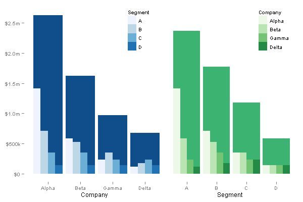
Ggplot2 Marimekko Replacement Overlapping Bars Data Visualization Design Information Visualization Graph Visualization

Data Visualization Charts 75 Advanced Charts In Excel Data Visualization Management Infographic Data Dashboard

Nevron Vision For Sharepoint Pie Chart Sharepoint Data Visualization Pie Chart

Probably The Only Way To Show Change Over Time In A Bar Chart Like The Greatest Growth Segmentation At The Top Data Design Data Visualization Bar Chart

R Ggplot2 How To Combine Histogram Rug Plot And Logistic Regression Prediction In A Single Graph Stack Overflow Logistic Regression Histogram Regression

Excel How To Create A Dual Axis Chart With Overlapping Bars And A Line Excel Excel Tutorials Circle Graph

Data Visualization Chart 75 Advanced Charts In Excel With Video Tutorial Data Visualization Visualisation Charts And Graphs

Dashboard Templates Data Visualization Charts And Graphs Dashboard Template Charts And Graphs Data Visualization

Multiple Width Overlapping Column Chart Peltier Tech Blog Data Visualization Chart Multiple

Pin On Others Peltier Tech